How Adam Steers Gradient Descent

Method	State	Update Rule	Comment
Vanilla GD	none	$\theta_{t+1}=\theta_t-\alpha \nabla f(\theta_t)$	Follow the gradient; can zig-zag in narrow valleys.
Momentum	$m_t$ for direction	$m_t=\beta m_{t-1}+(1-\beta)\nabla f(\theta_t)$ $\theta_{t+1}=\theta_t-\alpha m_t$	Build inertia: accelerate consistent directions, damp oscillations.
RMSProp	$v_t$ for scale	$v_t=\rho v_{t-1}+(1-\rho)(\nabla f(\theta_t))^{\odot 2}$ $\theta_{t+1}=\theta_t-\alpha\frac{\nabla f(\theta_t)}{\sqrt{v_t}+\epsilon}$	Per-parameter step size: large recent gradients → smaller steps.
Adam	$m_t$ and $v_t$	$\hat m_t=\frac{m_t}{1-\beta_1^t}$ $\hat v_t=\frac{v_t}{1-\beta_2^t}$ $\theta_{t+1}=\theta_t-\alpha\frac{\hat m_t}{\sqrt{\hat v_t}+\epsilon}$	Direction + normalization, with bias correction.

Momentum: building velocity

Fig 1. SGD without (left) and with (right) momentum.

Vanilla gradient descent: reactive, step-by-step

Let’s start from the most basic update rule. Suppose we want to minimize an objective $f(\theta)$. Vanilla gradient descent updates parameters by moving against the gradient:

$$ \theta_{t+1} = \theta_t - \alpha \nabla f(\theta_t) $$

where $\alpha$ is the learning rate.

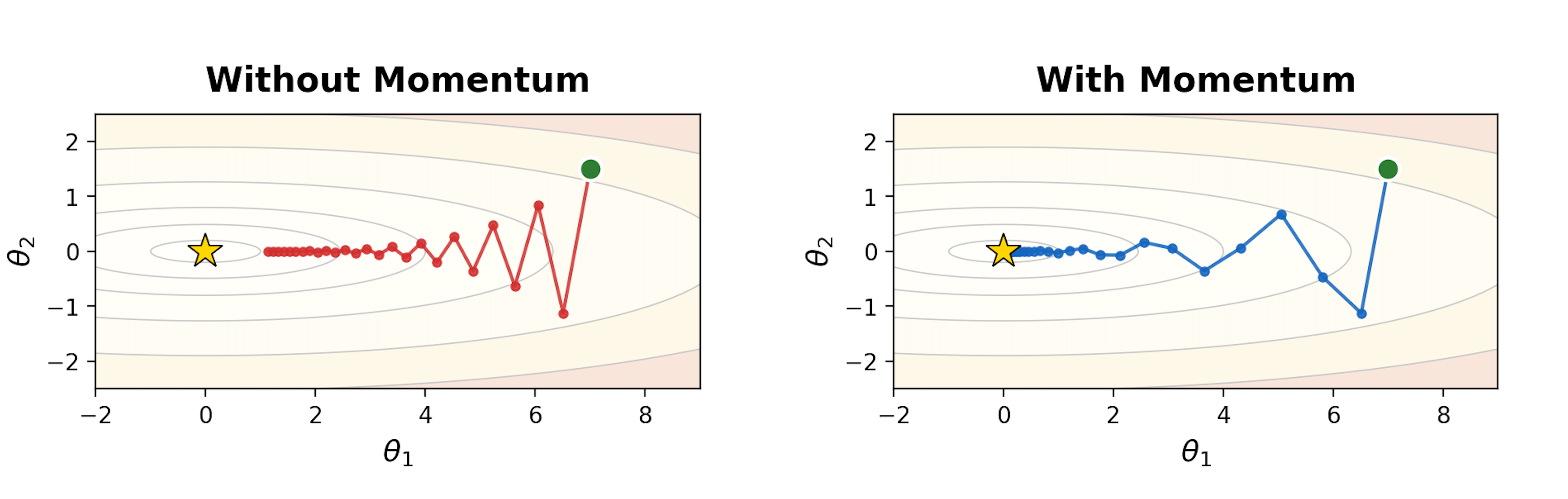
This rule is fully reactive: the step at time $t$ depends only on the current gradient. That can work, but it has a well-known failure mode in ill-conditioned landscapes (think “long narrow valleys”):

Along the steep direction, gradients are large → updates overshoot and flip sign.
Along the flat direction, gradients are small → progress is slow.
Net effect: zig-zagging and wasted steps (see Fig 1, left half).

A useful mental image: vanilla GD is like a person who looks at the slope under their feet each step and immediately turns to face the steepest downhill direction. In a narrow valley, they keep bouncing between the two sides instead of making steady progress along the valley floor.

A small idea: don’t forget the past

If gradients keep pointing in a roughly consistent direction (even if noisy), we can exploit that by accumulating them. Instead of directly using $\nabla f(\theta_t)$ as the step, we maintain a running direction that blends history with the present.

This is the core of momentum:

keep a momentum vector $m_t$,
update it as an exponential moving average of gradients,
update parameters using that momentum.

Gradient descent with momentum: add velocity

One common form (often called heavy-ball momentum [1]) is:

$$ m_t = \beta m_{t-1} + \nabla f(\theta_t), \quad \theta_{t+1} = \theta_t - \alpha m_t $$

where $\beta \in [0,1)$ is the momentum coefficient (often $0.9$).

Interpretation:

$m_t$ is a smoothed gradient: it keeps a memory of where gradients have been pointing.
When gradients are consistent, $m_t$ grows in that direction $\rightarrow$ accelerates progress.
When gradients oscillate (like across a valley wall), the positive/negative contributions partially cancel $\rightarrow$ damps zig-zagging.

You can also view this as an exponential moving average (EMA). Unrolling the recursion gives roughly:

$$ m_t \approx \sum_{k=0}^{t} \beta^{\,t-k} \nabla f(\theta_k) $$

so older gradients are still present, but exponentially down-weighted.

A concrete 1D toy example (sign flipping vs consistent signal)

Consider a 1D case.

If gradients are consistent: $\nabla f(\theta_t) = 1$ for many steps, then $m_t$ grows toward $\frac{1}{1-\beta}$:

$$ \lim_{t \rightarrow \infty} m_t \approx \lim_{t \rightarrow \infty} \sum_{k=0}^t \beta^{t-k} = \lim_{t \rightarrow \infty} \frac{1 - \beta^t}{1 -\beta} = \frac{1}{1-\beta} $$

so the effective step $\alpha m_t$ becomes larger than $\alpha$. You speed up.

If gradients flip: $\nabla f(\theta_t) = +1, -1, +1, -1, \dots$, then $m_t$ stays small because history cancels the present. You stop bouncing so hard.

This is exactly what we want in a narrow valley: don’t overreact to the steep direction that keeps flipping sign; instead, keep moving along the direction that stays consistent.

RMSProp: adaptive step sizes

Why momentum isn’t the full story

Momentum fixes a key weakness of vanilla gradient descent: it reduces zig-zagging by smoothing gradients over time and building a velocity in consistent directions.

But momentum still uses a single global learning rate $\alpha$ for all parameters and all directions. In many objectives, different coordinates can have very different curvature / gradient scales:

Some parameters consistently see large gradients (steep directions).
Others see tiny gradients (flat directions).
With one $\alpha$, you often face a tradeoff:
choose $\alpha$ small enough to avoid exploding in steep directions, but then learning is slow in flat directions;
or choose $\alpha$ larger for progress in flat directions, but risk instability elsewhere.

This motivates a second idea: scale the step size per-parameter based on how big recent gradients have been.

The core idea: normalize by recent gradient magnitude

RMSProp [2] maintains a running (exponentially-decayed) average of squared gradients.

Define a second-moment (variance-like) accumulator:

$$ v_t = \rho v_{t-1} + (1-\rho)\, \nabla f(\theta_t)^{\odot 2} $$

where $\nabla f(\theta_t)^{\odot 2}$¹Note 1$\cdot^{\odot p}$ denotes the element-wise power: $x^{\odot p} := \big(x_1^p,\;x_2^p,\;\ldots,\;x_d^p\big)$. means squaring each component of the gradient, and $\rho \in [0,1)$ is typically close to $1$ (e.g., $0.9$ or $0.99$).

Then update parameters by dividing by the root mean square of recent gradients:

$$ \theta_{t+1} = \theta_t - \alpha \frac{\nabla f(\theta_t)}{\sqrt{v_t} + \epsilon} $$

where $\epsilon$ is a small constant (e.g., $10^{-8}$) for numerical stability.

Intuition: “big gradients → smaller steps; small gradients → bigger steps”

Because of the denominator $\sqrt{v_t}$:

If a coordinate has large gradients consistently, $v_t$ becomes large, so the effective step size in that coordinate shrinks.
If a coordinate has small gradients consistently, $v_t$ stays small, so the effective step size becomes relatively larger.

So RMSProp behaves like an automatic, per-parameter learning-rate tuner: it helps stabilize steep directions without forcing the whole optimizer to slow down.

Relationship to AdaGrad

You can view RMSProp as a practical fix to AdaGrad.

AdaGrad accumulates squared gradients with a running sum, which can make learning rates decay too aggressively over long training.
RMSProp uses an exponential moving average instead of a sum, so it “forgets” old gradients and keeps learning rates from collapsing.

Adam: combining both

At this point we have two complementary ideas:

Momentum smooths gradients over time (keeps a running direction), reducing zig-zagging and helping consistent progress.
RMSProp rescales updates using a running average of squared gradients, giving per-parameter adaptive step sizes.

Adam (Adaptive Moment Estimation) [3] combines both by tracking:

a first-moment estimate (EMA of gradients), and
a second-moment estimate (EMA of squared gradients),

then using the ratio to form the update.

Step 1: Exponential moving averages of the 1st and 2nd moments

First moment (mean of gradients):

$$ m_t = \beta_1 m_{t-1} + (1-\beta_1)\,\nabla f(\theta_t) $$

Second moment (mean of squared gradients, element-wise):

$$ v_t = \beta_2 v_{t-1} + (1-\beta_2)\,(\nabla f(\theta_t))^{\odot 2} $$

$\beta_1$ plays the role of momentum (typical: $0.9$).
$\beta_2$ controls how slowly the second-moment estimate changes (typical: $0.999$).

Step 2: Apply bias correction

We usually initialize $m_0 = 0$ and $v_0 = 0$. Early in training, these EMAs are biased toward zero because they haven’t had time to “warm up”. Adam corrects this using:

$$ \hat{m}_t = \frac{m_t}{1-\beta_1^t}, \qquad \hat{v}_t = \frac{v_t}{1-\beta_2^t} $$

How does correction work?

For first momentum $m_t$, recall:

$$ m_t = \beta_1 m_{t-1} + (1-\beta_1)\nabla f(\theta_t), \qquad m_0=0 $$

Unrolling the recursion gives:

$$ m_t = (1-\beta_1)\sum_{i=1}^{t}\beta_1^{\,t-i}\,\nabla f(\theta_i) $$

If the gradients have approximately constant mean in early steps, $\mathbb{E}[\nabla f(\theta_i)] \approx \mu$, then

$$ \mathbb{E}[m_t] = (1-\beta_1)\sum_{i=1}^{t}\beta_1^{\,t-i}\mu = (1-\beta_1^t)\mu $$

So $m_t$ underestimates the mean by a multiplicative factor $(1-\beta_1^t)$.

Bias correction divides it out:

$$ \hat m_t := \frac{m_t}{1-\beta_1^t} \quad\Rightarrow\quad \mathbb{E}[\hat m_t] \approx \mu $$

The dividing factor $1/(1-\beta_1^t)$ approaches 1 as $t$ grows, so the correction fades out after early steps²Note 2This also resolves the “blow-up” worry: when $t$ is small, $m_t$ is also small (because it started at $0$), and the ratio mainly restores the scale of a proper weighted average..

The same logic applies to the second momentum $v_t$:

$$ v_t = \beta_2 v_{t-1} + (1-\beta_2)(\nabla f(\theta_t))^{\odot 2}, \qquad v_0=0 $$

yielding

$$ \mathbb{E}[v_t] \approx (1-\beta_2^t)\,\mathbb{E}\!\left[(\nabla f(\theta_t))^{\odot 2}\right], \qquad \hat v_t := \frac{v_t}{1-\beta_2^t} $$

Step 3: The Adam update

Finally, Adam updates parameters via:

$$ \theta_{t+1} = \theta_t - \alpha \frac{\hat{m}_t}{\sqrt{\hat{v}_t} + \epsilon} $$

This mirrors the “RMSProp normalization” idea, but replaces the raw gradient with a momentum-like direction $\hat{m}_t$.

What each term is doing

$\hat{m}_t$ is the smoothed direction (Momentum): it averages gradients so you don’t overreact to noisy mini-batches or oscillations.
$\sqrt{\hat{v}_t}$ is the scale normalizer (RMSProp): it shrinks steps where recent gradients have been large and allows relatively larger steps where gradients have been small.
Bias correction matters most at the beginning; later, $(1-\beta_1^t)$ and $(1-\beta_2^t)$ approach 1, so the correction fades out.

References

[1] B. T. Polyak. Some methods of speeding up the convergence of iteration methods. USSR Computational Mathematics and Mathematical Physics, 4(5):1–17, 1964.
[2] G. Hinton, N. Srivastava, K. Swersky. Neural Networks for Machine Learning — Lecture 6e: rmsprop. Coursera, 2012. (slides)
[3] D. P. Kingma and J. Ba. Adam: A Method for Stochastic Optimization. ICLR 2015. (arXiv:1412.6980)

Appendix: steepest descent

This appendix explains a key geometric fact used throughout optimization: At a point $\theta$, the gradient $\nabla f(\theta)$ points in the direction of steepest increase³Note 3The “steepest direction = gradient direction” statement is with respect to the Euclidean norm. If you measure step size with a different norm or metric, the “steepest” direction changes. of $f$, and its magnitude gives the maximum rate of increase.

Directional derivative: “how fast does $f$ change if I move this way?”

Take a small step from $\theta$ in some direction $u$ with $\|u\|_2 = 1$: $\theta(\epsilon) = \theta + \epsilon u$. The instantaneous rate of change of $f$ along direction $u$ is the directional derivative:

$$ D_u f(\theta) := \left.\frac{d}{d\epsilon} f(\theta+\epsilon u)\right|_{\epsilon=0} $$

Using a first-order Taylor expansion,

$$ f(\theta+\epsilon u) \approx f(\theta) + \epsilon \nabla f(\theta)^\top u $$

$$ D_u f(\theta) = \nabla f(\theta)^\top u $$

Why this is maximized by the gradient

We now ask: among all unit directions $u$, which one makes $D_u f(\theta)$ as large as possible?

This is a simple optimization problem: $\max_{\|u\|_2=1}\; \nabla f(\theta)^\top u$.

By the Cauchy–Schwarz inequality,

$$ \nabla f(\theta)^\top u \le \|\nabla f(\theta)\|_2 \, \|u\|_2 = \|\nabla f(\theta)\|_2 $$

and equality holds when $u$ is aligned with the gradient:

$$ u^\star = \frac{\nabla f(\theta)}{\|\nabla f(\theta)\|_2} $$

Therefore:

The steepest ascent direction is $u^\star = \frac{\nabla f(\theta)}{\|\nabla f(\theta)\|_2}$.
The maximum rate of increase (over all unit directions) is $\max_{\|u\|_2=1} D_u f(\theta) = \|\nabla f(\theta)\|_2$.

Why gradient descent uses the negative gradient

If the gradient points toward steepest increase, then the direction of steepest decrease is simply the opposite: $-\nabla f(\theta)$.

That’s why vanilla gradient descent updates parameters as:

$$ \theta_{t+1} = \theta_t - \alpha \nabla f(\theta_t) $$

Quick intuition

$\nabla f(\theta)$ encodes how sensitive $f$ is to changes in each coordinate.
Dotting with a direction $u$ projects that sensitivity onto the direction you plan to move.
The projection is largest when you move directly along the gradient.